Rendering
Of course, any plotting library needs a way to render figures for display, and Toyplot is no exception. To integrate Toyplot into your workflow as easily as possible, we provide four different rendering mechanisms:
Backends
At the lowest level, Toyplot provides a large collection of rendering backends. Each backend knows how to render a Toyplot canvas to a specific file format, and can typically render the canvas directly to disk, to a buffer you provide, or return the raw representation of the canvas for further processing. You choose a backend that provides the file format you want to generate, and use it to explicitly render your canvas. For example, you could use the toyplot.pdf backend to save a figure as a vector PDF image on disk:
import toyplot.pdf
toyplot.pdf.render(canvas, "figure1.pdf")
Similarly, you could substitute the toyplot.png backend to save a PNG bitmap image:
import toyplot.png
toyplot.png.render(canvas, "figure1.png")
You could do the same with the toyplot.svg backend, but suppose you wanted to add a custom CSS class to the SVG markup for inclusion in a publishing workflow. To accomodate this, the SVG backend can return a DOM for further editing, instead of saving it directly to disk:
import toyplot.svg
svg = toyplot.svg.render(canvas)
svg.attrib["class"] = "MyCustomClass"
import xml.etree.ElementTree as xml
with open("figure1.svg", "wb") as file:
    file.write(xml.tostring(svg))
Finally, there is Toyplot’s most important backend, toyplot.html which produces the preferred interactive HTML representation of a canvas. Like the other backends, you can use it to write directly to disk, or return a DOM object for editing as-needed:
import toyplot.html
toyplot.html.render(canvas, "figure1.html")
Note that the file produced by this backend is a completely self-contained HTML fragment that could be emailed directly to a colleague, inserted into a larger HTML document, etc.
Displays
While backends are useful when you wish to save a canvas to disk for incorporation into a paper or some larger workflow, in many cases you may find yourself simply wanting to display the results of some computation. Writing files to disk and opening them in a separate application can be time-consuming and frustrating, particularly when running a script repeatedly during development. For this case, Toyplot provides display modules, which provide convenient ways to display figures interactively. The most portable of these modules is toyplot.browser:
import toyplot.browser
toyplot.browser.show(canvas)
This will open a new browser window containing your figure, with all of Toyplot’s interaction and features intact.
Rich Display
For integration with Jupyter user interfaces such as Notebooks and Qt Consoles, the Toyplot canvas object provides rich display representations that can render it into a cell. For example, suppose you created a canvas using a Qt console:
In [1]: import numpy
   ...: import toyplot
   ...: x = numpy.linspace(0, 1)
   ...: y = x ** 2
   ...: canvas = toyplot.Canvas(width=300)
   ...: axes = canvas.cartesian()
   ...: mark = axes.plot(x, y)
To display the canvas, simply return it as the result of an expression, just as you’d inspect any other type:
In [2]: canvas
Out[2]:
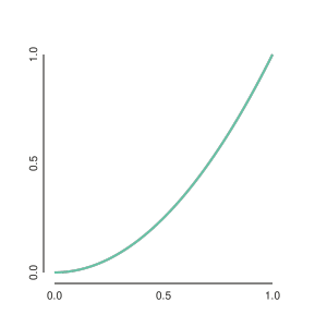
In the case of the Qt console, the figure is rendered as a PNG image and embedded in the cell output.
Autorendering
As a special case for interactive environments such as Jupyter notebooks, Toyplot’s autorender feature automatically renders a canvas into a notebook cell using Toyplot’s preferred interactive HTML representation. We use autorendering with few exceptions throughout this documentation. As an example, try running the same code from the previous example in two cells of a Jupyter notebook:
[1]:
import numpy
import toyplot
x = numpy.linspace(0, 1)
y = x ** 2
canvas = toyplot.Canvas(width=300)
axes = canvas.cartesian()
mark = axes.plot(x, y);
[2]:
canvas
[2]:
Now there are two copies of the figure! What happened is that autorendering automatically rendered the figure in the first cell, and then rich display worked as normal in the second cell. So, when using Toyplot in a notebook, you can leave out the second step. Note that no special import statements, magics, backends, or configuration is required - autorendering is enabled by default when you create a new canvas. Toyplot knows that it’s being run in the Jupyter notebook environment, and when
you execute a notebook cell that contains a canvas with autorendering enabled, it automatically inserts the rendered canvas in the cell output. The Toyplot canvas doesn’t have to be the result of an expression to be rendered, and you can create multiple Toyplot canvases in a single notebook cell (handy when producing multiple figures in a loop), and they will all be rendered in the cell’s output.
Autorendering for a canvas is automatically disabled when you pass it to a rendering backend or a display. So while the above example automatically rendered the canvas into a notebook cell, the following will not:
canvas = toyplot.Canvas(width=300)
canvas.axes().plot(x, y)
toyplot.pdf.render(canvas, "figure2.pdf")
If you want to write your figure to disk and see it in the notebook, just use rich display:
canvas = toyplot.Canvas(width=300)
canvas.axes().plot(x, y)
toyplot.pdf.render(canvas, "figure2.pdf")
canvas # To display the results in the notebook
In some circumstances you may want to disable autorendering yourself, which you can do when a canvas is created:
[3]:
canvas = toyplot.Canvas(width=300, autorender=False)
canvas.cartesian().plot(x, y);