Embedding
We like to say that “Toyplot figures are beautiful, scalable, embeddable, and interactive”, but what does embeddable really mean, anyway? Scientists and engineers are already accustomed to embedding static images in their publications and presentations, so what does embedding in Toyplot have to offer that other tools don’t?
In a word: interaction.
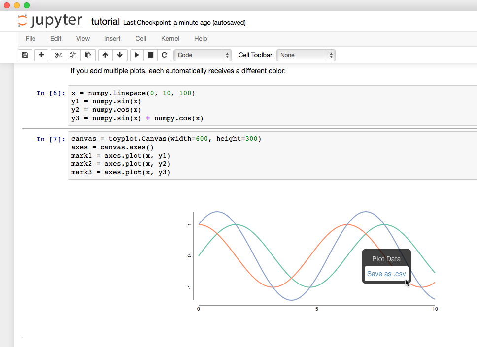
In their preferred HTML format, Toyplot figures are interactive - users can mouse over the figure to see interactive coordinates and even extract the data from a figure in CSV format using a context menu. This is just scratching the surface of what we want to achieve in interactivity, but the key point is that each figure is completely self contained and can be distributed as a single file without any need for a server, libraries, stylesheets, or even a network connection.
Here are some examples of Toyplot embedding in-action:
Jupyter (IPython) Notebooks
To use Toyplot in a Jupyter (IPython) notebook, simply import the library and create a plot - no extra statements, “magics”, or backend configuration required. The library knows that it’s being executed in the Jupyter environment, and automatically renders the plot into your notebook using the interactive HTML format:
“This is all well and good”, you may say, “and the interaction is nice, but it’s hardly a game-changer”.
But wait! This is where the self-contained nature of Toyplot figures really starts to shine. For example, if you use the notebook’s File > Download as > HTML (.html) menu command, your browser will download an HTML copy of the notebook, with the Toyplot figures embedded, as you might expect. What you might not expect is that the figures will still be live and interactive!
Slides
As another example, you can convert your Jupyter notebook into an interactive Reveal.js presentation using the nbconvert utility, and the embedded Toyplot figures in your slides will still be interactive during your presentation:
ipython nbconvert mynotebook.ipynb --to slides --post serve
Imagine being able to respond to audience questions with a live figure that was authored in a completely separate environment!
Documentation
Similarly, you can convert a Jupyter notebook to restructured text (the markup of choice for most Python documentation):
$ ipython nbconvert mynotebook.ipynb --to rst --output mynotebook.rst
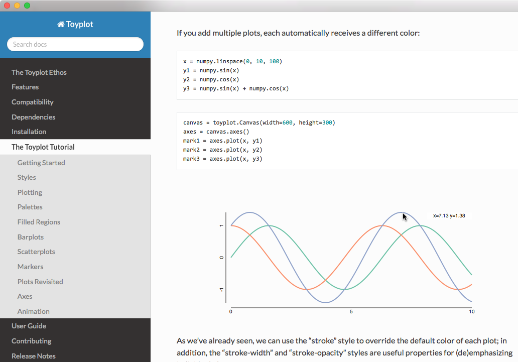
and the HTML Toyplot figures will be embedded in the restructured text and remain fully-interactive in the generated docs. This, by the way, is how much of the Toyplot documentation you’re reading right now is written - we author examples using Jupyter notebooks, which are converted to .rst files, then compiled into HTML documentation using Sphinx:
Electronic Publication
This leads to one of our key goals for Toyplot: supporting electronic publication, and changing what people expect from data graphics. Many scientific and engineering journals have begun to experiment with HTML-based publishing formats, and figures created with Toyplot are uniquely suited to the HTML publishing environment, providing useful interaction in a completely self-contained “package” that can be trivially inserted into an HTML document without introducing any other dependencies. Because Toyplot figures don’t rely on external servers, libraries or stylesheets, they can be embedded, copied, and moved from place-to-place where they will continue to Just Work without modification - properties that are critical for archival and accessibility.
E-Mail
Because a Toyplot figure is fully self-contained, it can be easily shared through e-mail or other electronic communication channels. You can e-mail a Toyplot figure to a colleague as an HTML file, and they will be able to easily view and interact with the file, in many cases right inside their e-mail client!
PyQT / PySide
Because the Qt graphical user interface includes a fully-featured WebKit browser and Python bindings (PyQt or PySide, take your pick), you can embed interactive Toyplot plots in just a few lines of code, with all the interaction intact:
window = QWebView()
canvas, axes, mark = toyplot.plot(x, y)
window.setHtml(xml.etree.ElementTree.tostring(toyplot.html.render(canvas), method="html"))
If you prefer, you could also embed static plots using the SVG or PNG backends:
window.setContent(xml.tostring(toyplot.svg.render(canvas)), "image/svg+xml")
or
window.setContent(toyplot.png.render(canvas), "image/png")
Programmatic Embedding
Toyplot provides a wide variety of Rendering backends in addition to the preferred, interactive HTML backend. The API implemented by the backends has been carefully crafted to support embedding and maximize consistency:
Most backends take a fileobj parameter in their render method. If you pass a string fileobj, the canvas will be written to the given filename on disk.
If you pass a file-like object as the fileobj parameter, the canvas will be written directly to the object. So you could store any figure to an in-memory
io.StringIObuffer for subsequent processing, for example.- If you don’t supply the fileobj parameter when rendering, the canvas will be returned to the caller in whatever high-level form is most appropriate for that backend:
The
toyplot.htmlandtoyplot.svgbackends return an instance ofxml.etree.ElementTree.Elementthat contains the DOM representation of the figure. This makes it easy to manipulate the figure for embedding in a larger DOM or subsequent processing.The
toyplot.pdfandtoyplot.pngbackends return the raw bytes of a PDF or PNG file, respectively. So you could pass the PNG image toPIL.Image.open(), for example.